Automatic disaggregation

Aggregation

Aggregation is a concept that has existed in routing protocols since the dawn of time. Aggregation allows a set of specific routes that all point to the same next-hop to be summarized by a single less specific route, called the aggregate route. For example, specific routes 10.1.0.0/16, 10.2.0.0/16, and 10.3.0.0/16 can be summarized by aggregate route 10.0.0.0/8 if they all have the same next-hop. Replacing all routes in the route table with a default route 0.0.0.0/0 (or ::0/0 in the case of IPv6) is an extreme example of aggregation.

The most common use case for aggregation is to reduce the size of the route table by removing unneeded details. For example, within their own network, Internet Service Providers (ISPs) need specific routes to each of their customers. However, ISPs typically only advertise a single aggregate route for their entire address space to other ISPs.

Most existing routing protocols (BGP, OSPF, ISIS, …) support manual configuration of aggregation.

Disaggregation

The concept of disaggregation has been around for a long time as well. Disaggregation is the opposite of aggregation: it takes a single less specific route (the aggregate route) and splits it up into several more specific routes.

The most common use case for disaggregation is traffic engineering. For example, an enterprise that is BGP dual-homed to two service providers may split its address space (described by an aggregate) into two more specific prefixes, and advertise one to each service provider. That way, incoming traffic is split across the two service providers, even if one service provider has a shorter incoming path than the other.

Most existing routing protocols (BGP, OSPF, ISIS, …) provide mechanisms to manually configure disaggregation. There exist so-called BGP optimizers that automatically configure BGP disaggregation for traffic engineering purposes. These are separate appliances, not something that is built into the BGP protocol itself.

RIFT automatic disaggregation

In this feature guide we explain how automatic disaggregation is implemented in RIFT.

In most existing protocols (BGP, OSPF, ISIS) disaggregation requires extensive manual configuration. In RIFT, by contrast, disaggregation is fully automatic without the need for any configuration.

In most existing protocols, disaggregation is an optional and manual feature that is mainly used for traffic engineering. RIFT, on the other hand, relies on disaggregation as an essential feature to recover from failures. In the absence of a failure, RIFT routers only have a default route for the north-bound direction. When a failure occurs, RIFT automatically triggers necessary disaggregation to install more specific north-bound routes to route traffic around the failure.

There are actually two flavors of disaggregation in RIFT:

• Positive disaggregation is used to deal with most types of failures. It works by the repair path “attracting” traffic from the broken path by advertising more specific routes. Positive disaggregation in RIFT works very similar to how disaggregation works in existing protocols, except that it is triggered automatically instead of configured manually.

• Negative disaggregation is used to deal with a very particular type of failure that only occurs in large data centers, so-called multi-plane fat trees (we will explain what multi-plane means later on). Negative disaggregation works by the broken path “repelling” traffic towards the repair path by advertising so-called negative routes. Negative disaggregation uses completely new mechanisms that (as far as we know) do not have an equivalent in any widely deployed existing protocols.

In this guide we describe how both of these flavors of disaggregation work from a RIFT protocol point of view (i.e. not tied to any particular implementation). The following two feature guides describe the command-line interface (CLI) for disaggregation in the RIFT-Python open source implementation. Both of these documents contain lots of concrete examples that help you translate the theory in this paper into actual hands-on practical experience:

• The RIFT-Python positive disaggregation feature guide.

• The RIFT-Python negative disaggregation feature guide.

Since RIFT relies on positive disaggregation to reroute traffic after a failure, positive disaggregation is always enabled in RIFT; it is not an optional feature and it cannot be disabled.

Negative disaggregation is a bit more subtle. As we will see later in this paper, certain aspects of negative disaggregation (“origination”) are only needed in certain topologies (“multi-plane fabrics”) and only in certain parts of the network (“top-of-fabric nodes”). For that reason, an implementation may choose to only partially support negative disaggregation.

Terminology

A quick note on terminology used in this paper before we proceed:

• A node is synonymous with a router or layer 3 switch.

• A fabric is synonymous with a network.

• We use terms leaf, spine, and superspine for the layers of nodes in a 3-level fat tree fabric.

• A top-of-fabric (ToF) node is the highest node in the hierarchy. In a 2-level fabric the spine nodes are the top-of-fabric nodes. In a 3-level fabric the superspine nodes are the top-of-fabric nodes.

• A point-of-delivery (PoD) is a group of nodes that is only north-south connected to nodes higher in the fabric hierarchy and not east-west connected to other pods. A pod can be thought of as a “logical node” and is typically deployed as a unit.

• A top-of-pod (ToP) node is the highest node in each pod. In 3-level fabrics, each pod normally has 2 levels and the spine nodes are the top-of-pod nodes. In extremely large 4- or 5-level fabrics, the pods themselves can be more than 2 levels. Running RIFT on the servers to support dual-homing increases the level of pods by one.

• To be consistent with current networking literature, we treat fat tree topologies as roughly synonymous with Clos topologies (although Clos topologies are historically a circuit-switching concept, Clos topologies never have east-west links, and in Clos topologies all links have the same capacity).

• A 2-level fat tree topology corresponds to a 3-stage Clos topology, a 3-level fat tree topology corresponds to a 5-stage Clos topology, etc.

RIFT route tables in the absence of failures

As mentioned before, one of the best-known characteristics of RIFT is that it is a link-state protocol north-bound and a distance-vector protocol south-bound. One consequence of this is that the RIFT route tables typically contain:

• Specific routes for all south-bound traffic. These are typically host /32 (for IPv4) or /128 (for IPv6) routes, but it could be something less specific as well.

• Fabric default routes for all north-bound traffic. These are typically 0.0.0.0/0 and ::0/0, but it could be something more specific as well.

Figure 1 below shows typical RIFT route tables in a small 3-level fabric. The leaf nodes contain only a single north-bound default route. The superspine nodes contain only host-specific south-bound routes. And the spine nodes contain a mixture.

To keep the figures simple and readable, this figure (and subsequent figures) only show the node loopback prefixes. In the real world, fabric addressing is a bit more complicated:

• The link interfaces would also have IP addresses (which are not shown in the figures). In IPv6 these would typically be automatically assigned link-local addresses. In IPv4 these would typically be manually assigned /31 prefixes. Alternatively, IPv4 could use the technique described in RFC5549 to use IPv6 link-local next-hops for IPv4 prefixes. The link interface prefixes are typically not advertised in RIFT; they are only used locally as next-hops and for sending RIFT messages.

• In a real fabric there would be a rack of servers attached to each leaf node. Those servers could be bare-metal servers or they could host virtual machines or containers. The servers could also run RIFT; in that case the servers are the leaf nodes. If the servers are dual-homed host-based RIFT provides automatic recovery when one of the dual-homing links or top-of-rack switches fails.

• If the network is flat (i.e. no overlay is used) then the leaf nodes would also advertise the server addresses and/or the addresses of the virtual machines or containers.

• If the network uses overlays, RIFT would also advertise the overlay tunnel end-points, which may be located on the leaf nodes or on the servers.

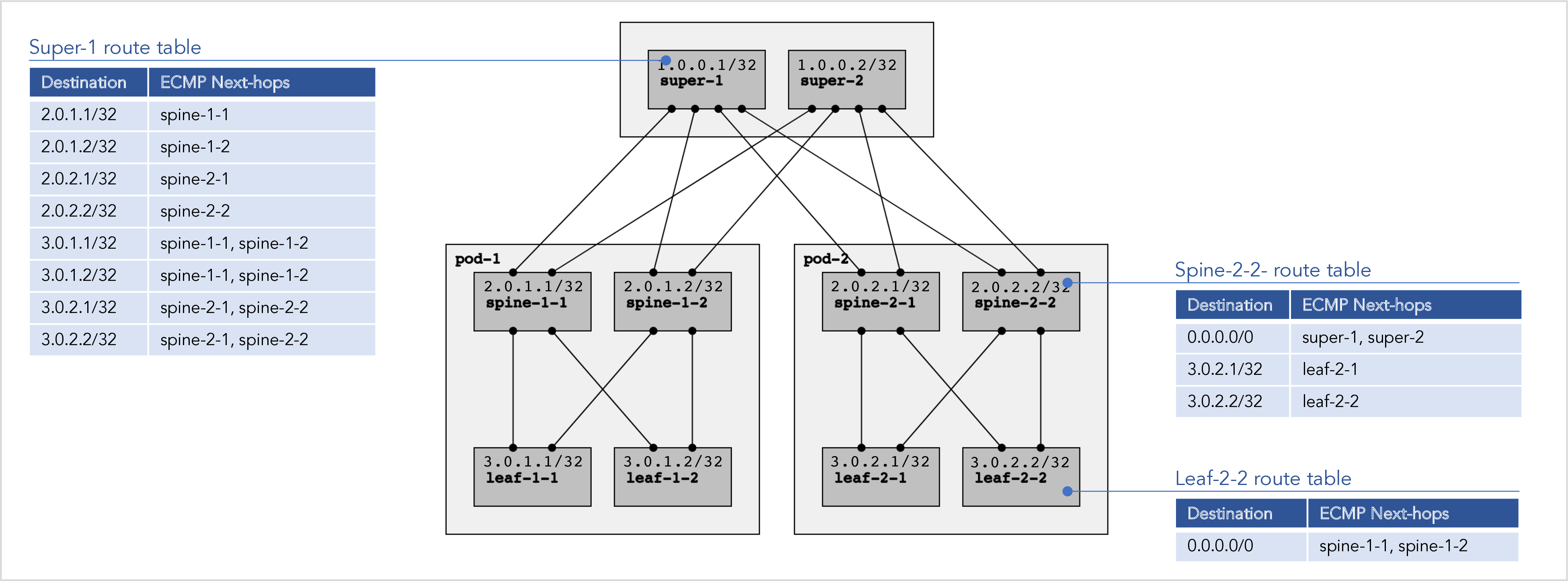
Figure 1: Typical RIFT route tables in the absence of failures.

If there are no failures (no broken links and no broken nodes) anywhere in the topology, then default routes work just fine. Each node can just “spray” all north-bound traffic across all parent nodes using an equal cost multi-path (ECMP) default route. In fact, since RIFT is a valley-free routing protocol (i.e. inherently loop-free) any desired weights can be used; it does not have to be equal cost. The fat tree topology guarantees that (in the absence of failures) it doesn’t matter which parent node is chosen: any parent node is able to reach the final destination, typically at the same cost as any other parent node.

As a concrete example, consider the traffic from leaf-1-1 to leaf-2-2 in figure 1 above. Leaf-1-1 can pick either spine-1-1 or spine-1-2 as the next-hop for sending traffic to leaf-2-2. It doesn’t matter which spine leaf-1-1 picks. Both spine-1-1 and spine-1-2 have a path to leaf-2-2, and one path is no better than the other (they are equal cost). Everything we have said is not only true for destination leaf-2-2, but for any destination leaf. For that reason, leaf-1-1 only needs a default route with ECMP next-hops spine-1-1 and spine-1-2.

Similarly, spine-1-1 can send traffic destined for leaf-2-2 to either super-1 or super-2. Once again it doesn’t matter. So, once again, the spines only need multi-path default routes for north-bound traffic.

RIFT TIE messages in the absence of failures

Consider the following leaf-spine fabric:

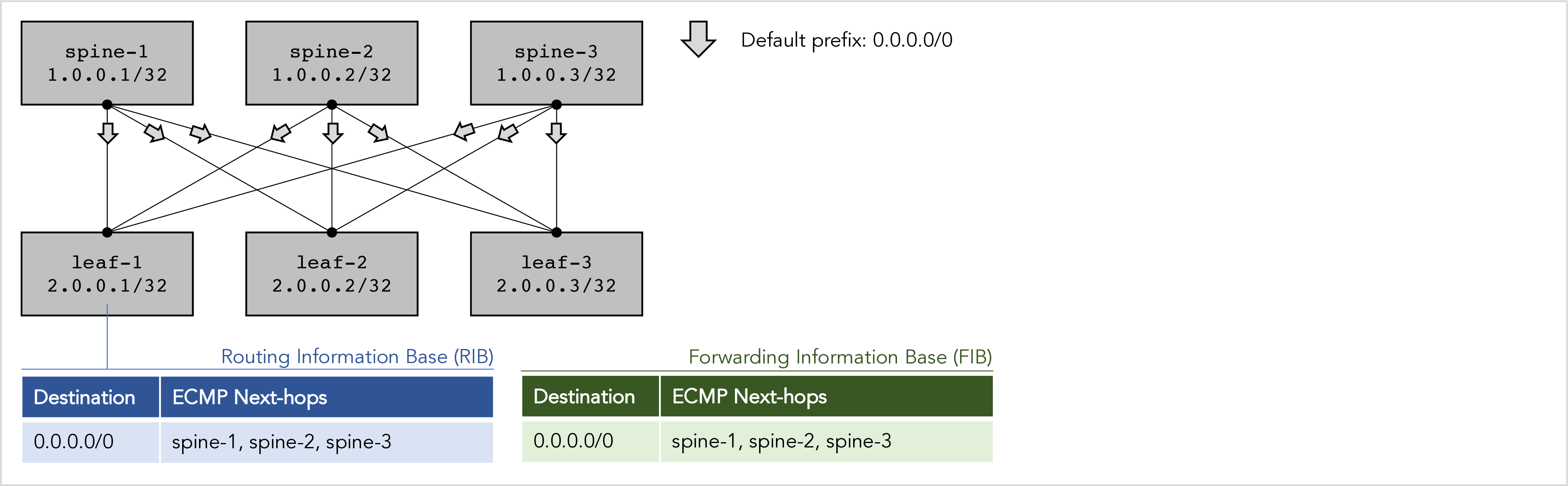
Figure 2: In the absence of failures RIFT advertises a default route.

The following sequence of RIFT messages leads to the installation of a default north-bound route in the Routing Information Base (RIB) and Forwarding Information Base (FIB) of each leaf node.

1. All the RIFT nodes have exchanged link information element (LIE) messages and have established adjacencies. RIFT LIE messages are similar to OSPF hello packets.

2. Then, each spine node sends a south prefix topology information element (TIE) message to each of the leafs to advertise a default route. RIFT TIE messages are similar to OSPF link state update packets (although the flooding rules in RIFT are quite different).

3. Thus, each leaf node receives a south prefix TIE with a default route from each of its spine nodes.

4. This results in each leaf node installing a multi-path default north-bound route that “sprays” all traffic over all three spine nodes. The multi-path default route is typically an equal-cost multi-path (ECMP) route, but if bandwidth weighting is used, it could be a weighted equal-cost multi-path (WECMP) route as well. Technically, we could say that the route is a result of the leaf running a north-bound Shortest Path First (SPF) algorithm, but since south TIEs are not propagated, it is a trivial SPF.

RIFT also has messages to make the TIE flooding reliable. RIFT topology information description element (TIDE) messages are similar to OSPF database descriptor packets, and RIFT has topology information request element (TIRE) messages are similar to OSPF link state request and link state acknowledgement packets combined.

Make a mental note of the fact that the traffic from leaf-1 to leaf-3 is spread equally across all three spine nodes. This will turn out to be important later on. (We are assuming here that the traffic consists of a sufficient number of flows, allowing ECMP hashing to do its job.)

RIFT disaggregation triggered by failures

Needing only default routes in the happy case of no failures is all good and well, but we have to consider the unhappy scenario as well. What if one or more links or nodes are down? In this case a simple default route for all north-bound traffic is not going to work.

Automatic disaggregation (either the positive or the negative flavor) is RIFT’s mechanism for recovering from failures by installing more specific routes to circumvent the failure. The word disaggregation is simply a fancy word for using a more specific route instead of the default route.

To figure out how automatic disaggregation works exactly, we must delve into the following questions:

• How does RIFT know a failure occurred?

• How does RIFT know which destination prefixes are broken and need to be repaired using disaggregation?

• How does RIFT figure out what alternative path to use to circumvent the traffic around the failure?

• How does RIFT decide whether to use positive disaggregation (i.e. attract traffic towards the repair path) or negative disaggregation (i.e. repel traffic away from the broken path)?

• What is the exact mechanism that positive disaggregation uses to attract traffic towards the repair path?

• What is the exact mechanism that negative disaggregation uses to repel traffic away from the broken path?

We shall answer these questions separately for positive and negative disaggregation.

RIFT positive disaggregation

Positive disaggregation on the spine nodes

We will explain how positive disaggregation works using the following example, where the link between spine-1 and leaf-3 fails as indicated by the red cross:

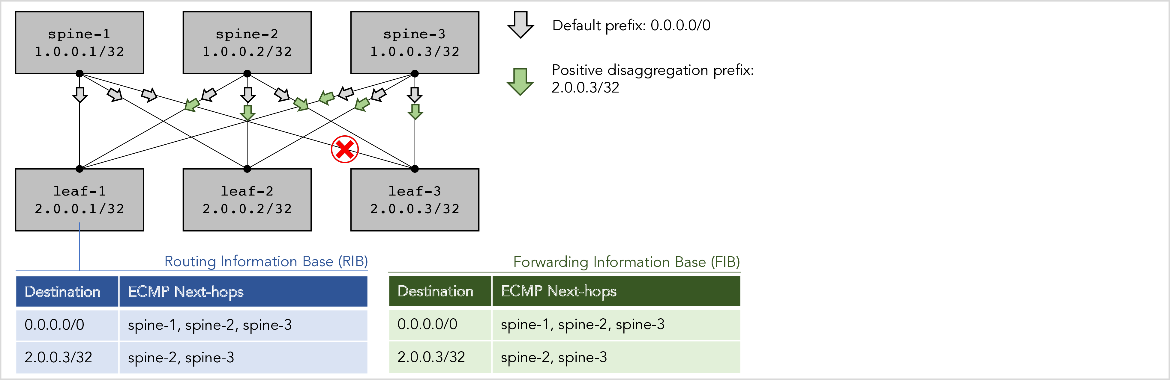
Figure 3: Positive disaggregation repairs a failure in a 2-level fabric.

The first thing to observe is that having only a default route on leaf-1 is not good enough anymore. Why not? Let’s see what happens if leaf-1 sends a packet to leaf-3. Assuming ECMP, the default route has a 1/3rd chance of sending the packet to spine-1, a 1/3rd chance for spine-2, and a 1/3rd chance for spine-3. If it happens to choose spine-1, the packet will be dropped, because spine-1 cannot get to leaf-3.

Well, technically speaking there are physical paths from spine-1 to leaf-3 (for example spine-1 -> leaf-2 -> spine-2 -> leaf-3) but that requires going back south and then north again (also known as “trombone routing”), which RIFT carefully avoids to maintain its valley-free and loop-free properties.

Positive disaggregation detects and recovers from this failure as follows:

1. Spine-2 knows exactly which south-bound adjacencies spine-1 has. This is because spine-1’s south node TIE, which reports spine-1’s adjacencies, is “reflected” by the leaf nodes to spine-2.

2. Spine-2 inspects the next-hops for each of its own south-bound routes. Let’s say spine-2 looks at the south-bound route for prefix P with next-hops NH1, NH2, …, NHn. Spine-2 then asks itself the question: “Can spine-1 also reach prefix P?”. Answering this question does not require any complicated computations; it is sufficient for spine-2 to examine the list of spine-1’s adjacencies.

3. The answer is “Yes, spine-1 can reach prefix P” if spine-1 has an adjacency to at least one of the next-hops NH1, NH2, …, NHn. In this case spine-2 does nothing.

4. The answer is “No, spine-1 cannot reach prefix P” if spine-1 does not have any adjacency to any of the next-hops NH1, NH2, …., NHn. In this case, spine-2 triggers positive disaggregation:

   a. Spine-2 uses a “south positive disaggregation prefix TIE” to advertise the specific prefix P south-bound to all leaves. In this example, spine-2 advertises prefix 2.0.0.3/32 to all leaves.

   b. Each of the leaves runs a north-bound Shorted Path First (SPF), which results in a route to P (2.0.0.3/32) being installed in the route table, with spine-2 as the next-hop.

   c. Since this route is more specific than the default route, all leaves will start sending traffic for destination prefix P to spine-2 instead of following the default route.

   d. The net effect of this is that spine-2 “attracts” the traffic away from the failed link on spine-1.

5. Spine-3 does the exact same thing as spine-2: it also looks for broken links on spine-1 and routes around those failures using positive disaggregation. In general, every node is constantly monitoring every other node at the same level in this manner. After this example has fully converged, the leaf nodes will end up with an ECMP route for destination leaf-3 (i.e. for prefix 2.0.0.3/32) that ECMPs the traffic across spine-2 and spine-3 (but not spine-1) as next-hops.

Note that step 5 takes place independently and asynchronously on each spine node. Thus, as the positive disaggregation process is converging, the host-specific positive disaggregation route starts out with a single next-hop, then two ECMP next-hops, until it finally ends up with N-1 ECMP next-hops where N is the number of spine nodes.

This can be a problem. The traffic that used to be spread out over N nodes is temporarily concentrated on a single spine node, then two spine nodes, until it is finally spread out over N-1 spine nodes again. This is referred to as the “transitory incast” problem. Various implementation techniques can alleviate this issue. Later we will see how negative disaggregation avoids this problem completely.

Positive disaggregation on the superspine nodes

We now consider positive disaggregation in a more complex scenario, namely a 3-level fabric. First we consider a single failure, namely the super-1 to spine-1-3 link marked with the red cross in figure 4 below. In this single-failure scenario:

• Both super-2 and super-3 advertise a positive disaggregation prefix for spine-1-3 (prefix 2.0.1.3/32) because they detect that super-1 cannot reach spine-1-3 anymore.

• However, they do not advertise a positive disaggregation prefix for leaf-1-1 (3.0.1.1/32), leaf-1-2 (3.0.1.2/32), or leaf-1-3 (3.0.1.3/32) because spine-1 can still reach those leaves via other spine nodes (namely via spine-1-1 or spine-1-2).

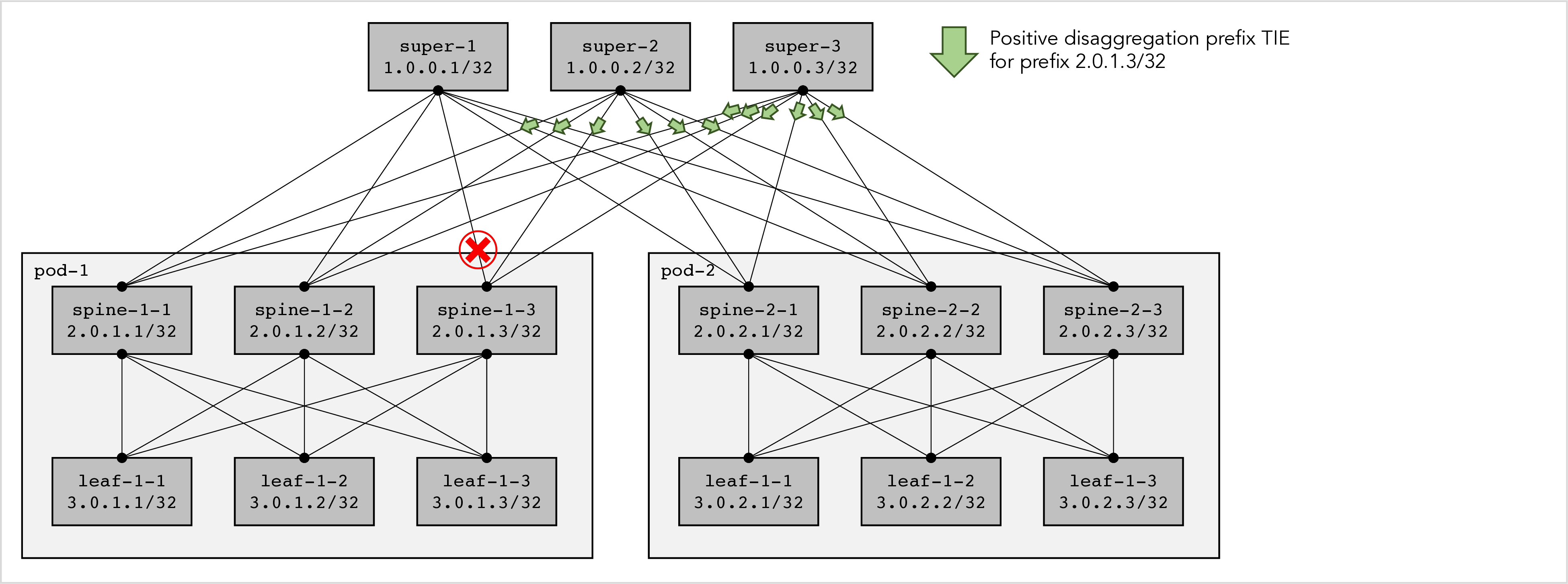
Figure 4: Positive disaggregation repairs a single failure in a 3-level fabric.

Next, we consider a scenario with three failures that completely disconnects super-1 from pod-1, as shown in figure 5 below. In this scenario both super-2 and super-3 advertise positive a disaggregation prefix TIE that reports all prefixes in pod-1, because they detect that super-1 cannot reach any spine next-hop in pod-1 anymore.

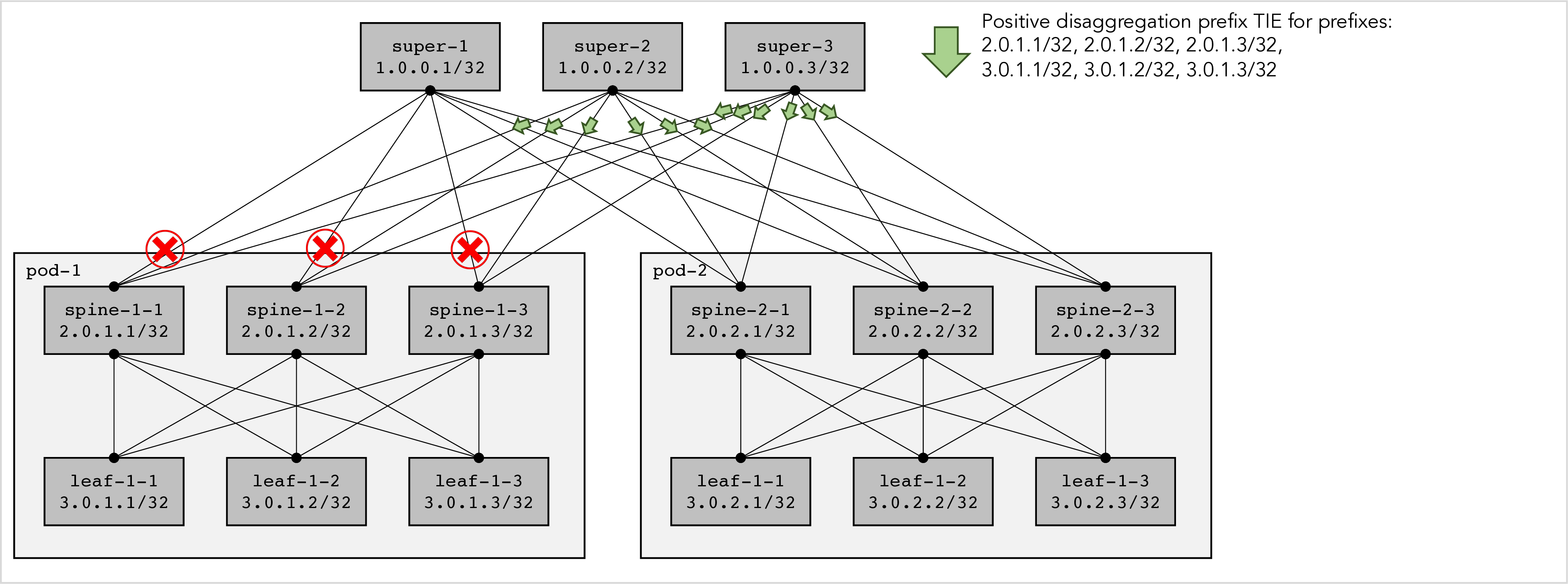
Figure 5: Positive disaggregation repairs a disconnected pod in a 3-level fabric.

Positive disaggregation prefix TIEs are non-transitive: when a spine receives a positive disaggregation prefix TIE from a superspine, it does not propagate the TIE further south-bound to the leaves. Each level in the fabric makes its own independent decision about which prefixes need to be positively disaggregated in the level below.

RIFT negative disaggregation

Why is negative disaggregation needed?

In the vast majority of topologies and failure scenarios, RIFT only needs positive disaggregation to recover from link and node failures. However, in one particular topology, namely the multi-plane topology, positive disaggregation does not work for some failure scenarios, for example the one shown in figure 6 below:

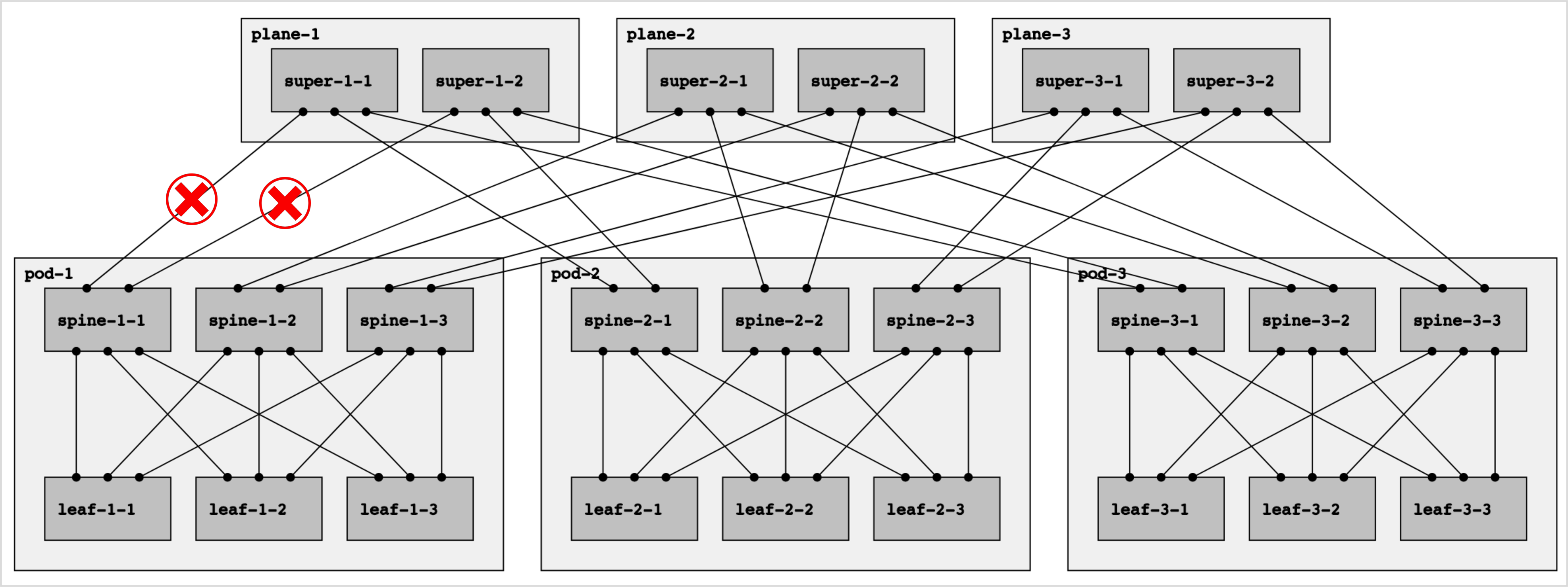
Figure 6: The need for negative disaggregation in multi-plane topologies.

The above topology is called a multi-plane topology because each spine in a pod is connected to a separate “plane” of superspine nodes. This reduces the number of ports that is needed on the superspine nodes. The following 3-dimensional representation of the same topology makes it more clear why this is called a multi-plane topology (the different colors represent different planes):

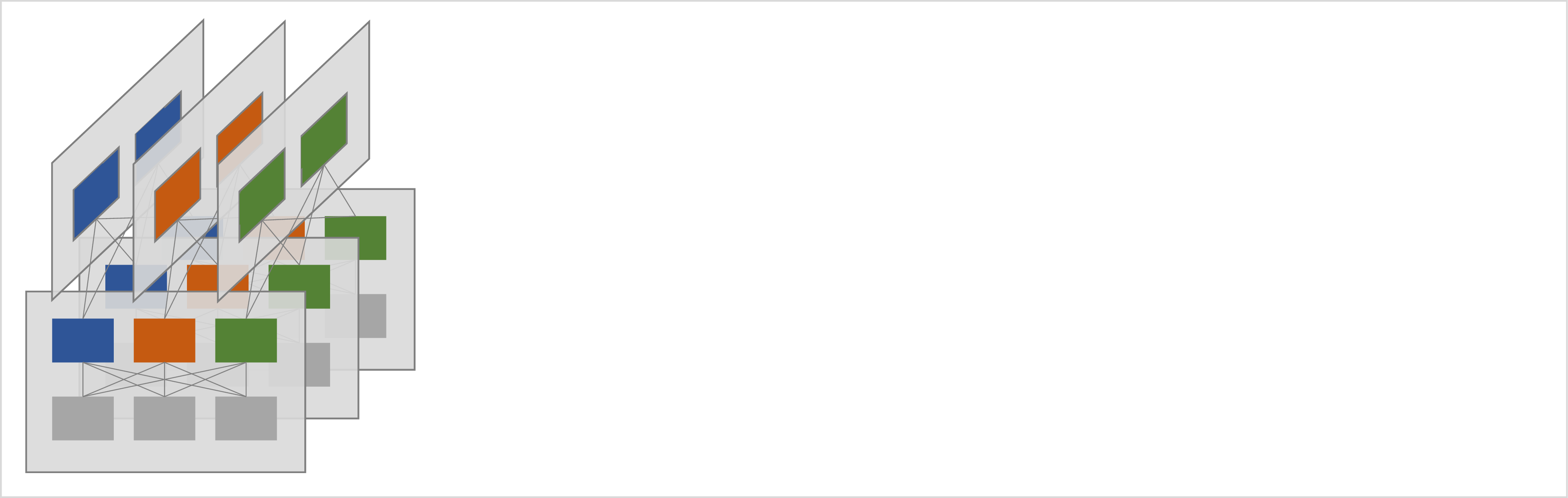
Figure 7: A multi-plane topology (3-dimensional representation).

Note that multi-plane topologies are only needed in large data centers with low radix core switches, i.e. if the switches that interconnect the pods do not have enough ports to connect to every top-of-pod switch in every pod.

Consider the scenario where the two links marked with red crosses in figure 6 above have failed, and consider traffic from leaf-2-2 to leaf-1-1:

• Leaf-2-2 has a north-bound default route with spine-2-1, spine-2-2, and spine-2-3 as ECMP next-hops.

• Let’s say leaf-2-2 picks spine-2-1 as the next-hop (there is a 1 in 3 chance that this happens).

• Since spine-2-1 is in plane-1, it has a north-bound default route with super-1-1 and super-1-2 as ECMP next-hops (these are the superspines in plane-1).

• At this point it doesn’t matter anymore which next-hop spine-2-1 picks: neither super-1-1 nor super-1-2 are able to reach leaf-1-1.

• The traffic from leaf-2-2 to leaf-1-1 the traffic is blackholed.

Note that the traffic from leaf-2-2 to leaf-1-1 was already doomed after leaf-2-2 chose spine-2-1 as the first next-hop. At that point the traffic entered plane-1. But the failures have completely disconnected plane-1 from pod-1. As soon as the traffic enters plane-1 it cannot reach any node in pod-1 anymore (once again, keeping in mind that tromboning is not allowed).

Positive disaggregation cannot save the day in this scenario. None of the spine nodes are sending any negative disaggregation prefixes to any of the leaves because there are no broken adjacencies below any of the spines. And the superspines are also not generating any positive disaggregation prefixes in this scenario, and even if they did, they would not be propagated to the leaves.

We will now describe how negative disaggregation fixes this problem.

Negative disaggregation is the opposite of positive disaggregation

As we have seen, positive disaggregation consists of two steps:

1. Node A detects that some other node B at the same level is unable to reach some south-bound prefix P. Nodes A and B can be at any level except the leaf level.

2. Node A originates a south-bound positive disaggregation prefix P to “attract” the traffic for P to itself. As a result of this traffic for P prefers node A (the repair path) over node B (the broken path).

Negative disaggregation works in the opposite way:

1. Node A detects that it itself is unable to reach some south-bound prefix P that some other node B at the same level is able to reach. Nodes A and B must be top-of-fabric nodes with inter-plane east-west links.

2. Node A originates a south-bound negative disaggregation prefix P to “repel” the traffic for P away from itself, i.e. away from node A. As a result, traffic for P prefers node B (the repair path) over node A (the broken path).

Later, towards the end of this paper, we will see that negative disaggregation is an abstraction that exists only in the control-plane. The data-plane only uses traditional (positive) routes. We will explain how abstract negative routes are translated into normal positive routes before they are installed into the data-plane.

Note: The data-plane of a router is the subsystem that actually forwards the packets. The data-plane can be hardware, e.g. an application specific integrated circuit (ASIC), or it can be software, e.g. the Linux kernel. The data-plane is controlled by the control-plane which is the software running the routing protocols and programming the forwarding tables. The word “plane” in data-plane and control-plane has nothing to do with the planes in a multi-plane fabric.

Triggering negative disaggregation

How does a top-of-fabric node A detect that it itself is unable to reach some prefix P that another top-of-fabric node B is able to reach? In other words, what is the trigger for negative disaggregation?

To make this possible, RIFT requires that the planes in the top-of-fabric are connected to each other using east-west inter-plane rings as shown in figure 8 below:

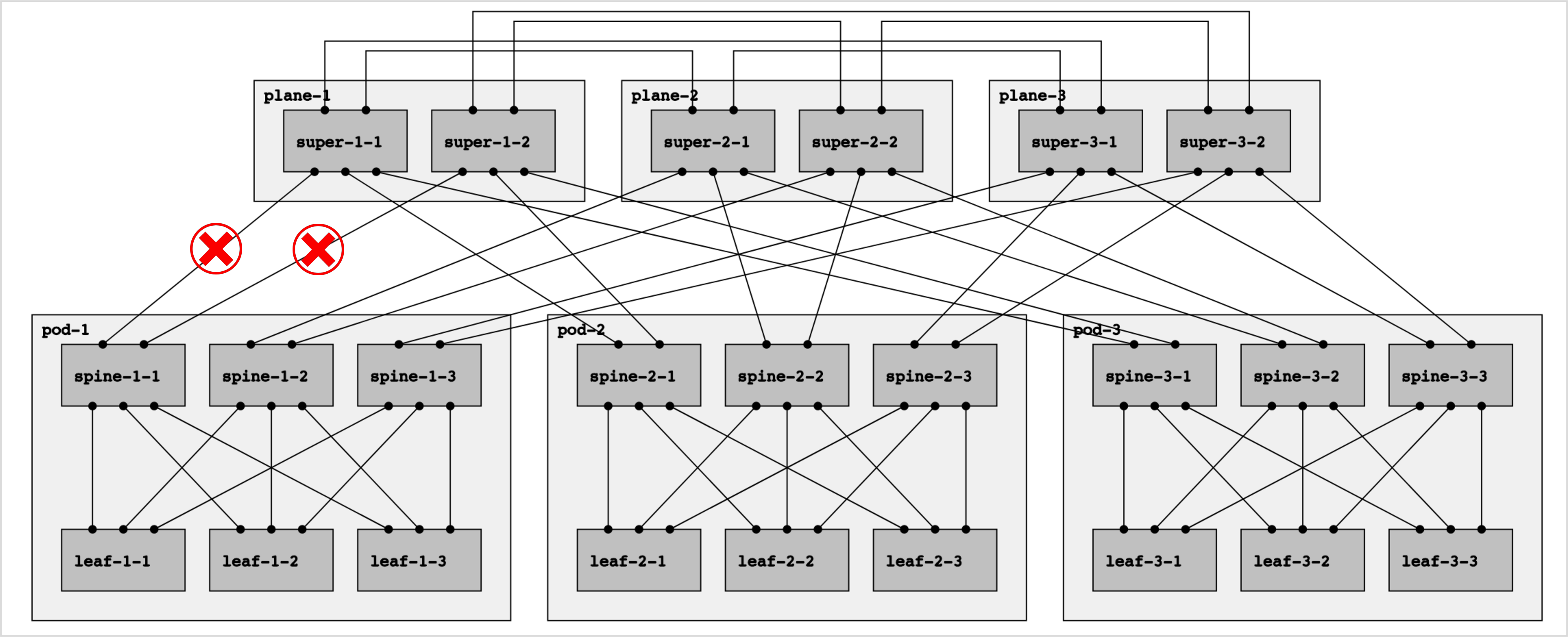
Figure 8: A multi-plane topology with east-west inter-plane links.

Note that there are two “rings” that interconnect the planes: one ring containing super-1-1, super-2-1, and super-3-1, and another ring containing super-1-2, super-2-2, and super-2-3. As a result, each superspine node requires exactly two east-west links, independently of the fabric size. (Obviously multiple parallel links can be used to make the ring more resilient.)

In the three-dimensional representation it is a bit more clear why these are called rings:

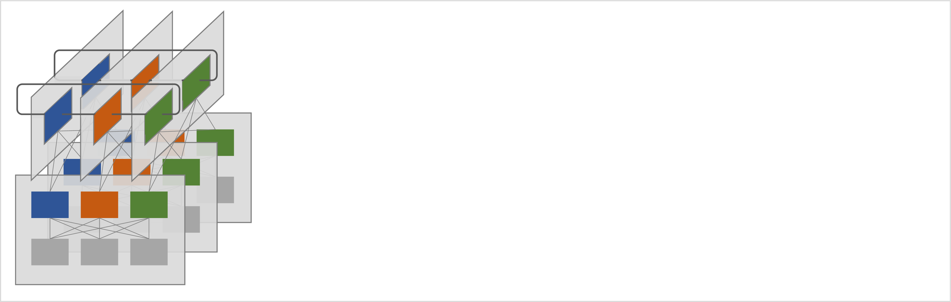
Figure 9: A multi-plane topology with east-west inter-plane links (3-dimensional representation).

These east-west inter-plane rings are normally not used to carry end-user payload traffic; they are only used to carry certain types of RIFT routing protocol messages. As a result, these can be low-bandwidth links (e.g. 1 Gbps instead of 100 Gbps).

The RIFT messages that are exchanged over these inter-plane east-west links include LIE messages for establishing adjacencies and a subset of the TIE/TIDE/TIRE messages flooding a subset of the link-state. The RIFT scoped flooding rules give the exact details, but the important point is that all north TIEs are also flooded over these east-west links. This allows a top-of-fabric node in one plane to discover the topology of all the other planes, but only for the purpose of triggering negative disaggregation, not for the purpose of actually sending end-user payload traffic to other planes over the east-west links (which, although possible, would largely negate the highly desirable property of fabrics uniformly and predictably spreading the traffic across all available links).

Normally, when RIFT runs a shortest path first (SPF) calculation to compute the shortest path to each destination prefix, it does not include these top-of-fabric inter-plane east-west links in the SPF topology. As far as the normal SPF is concerned, these links do not exist. This is what prevents these links from being used for end-user payload traffic.

However, for the purpose of negative disaggregation, RIFT runs an extra south-bound SPF calculation in which these top-of-fabric inter-plane east-west links are included. The results of this special SPF calculation are not used to populate the route tables. Instead, the result is only used to trigger negative disaggregation.

This extra SPF is only run on top-of-fabric nodes that have at least one east-west interface. It is not run on another type of node, and as an optimization it can be skipped if the top-of-fabric node does not have any east-west interfaces (and, obviously, also on any node that is not a top-of-fabric node).

The top-of-fabric nodes compare the reachable prefixes that are discovered by the normal south-bound SPF run with the reachable prefixes that are discovered by the special south-bound SPF run that includes inter-plane east-west links.

It is possible that the special SPF run discovers some extra reachable prefixes that were not reachable in the normal SPF run. This is because (as we mentioned above) north TIEs are also flooded over the east-west links. In that set of extra reachable prefixes, negative disaggregation only considers prefixes that are advertised by leaves. Extra prefixes that are originated by spine or superspine nodes are discarded for technical reasons that we won’t get into. The final set of discovered extra reachable leaf prefixes is known as “the fallen leaves”.

The fallen leaf prefixes are exactly the set of prefixes that we are interested in: it is the set of prefixes that the current top-of-fabric node cannot reach in the current plane, but that is reachable in at least one other plane.

For example, in the topology in figure 8 above where the two links with red crosses are down:

• Super-1-1 cannot reach leaf-1-1 in the normal SPF run, i.e. using only north-south links.

• However, super-1-1 can reach leaf-1-1 in the special SPF, by using an east-west link. One feasible route is super-1-1 -> super-2-1 -> spine-1-2 -> leaf-1-1.

Super-1-1 has discovered that leaf-1-1 is a fallen leaf. What this really means is that spine-1-1 has discovered that:

• Leaf-1-1 exists in the topology.

• Super-1-1 itself cannot reach leaf-1-1 using plane-1.

• At least one top-of-fabric node in another plane can reach leaf-1-1.

• This is what triggers super-1-1 to initiate negative disaggregation of all prefixes originated by leaf-1-1 (we describe what that means in the next section).

Leaf-1-1 is not the only fallen leaf. Using the same reasoning as above, we can see that leaf-1-2 and leaf-1-3 are also fallen leaves in plane-1. So, super-1-1 will also initiate negative disaggregation for their prefixes.

Super-1-1 is not the only top-of-fabric node that discovers these fallen leaves. Super-1-2 also discovers the same fallen leaves using the same procedure. So, super-1-2 will also initiate negative disaggregation for fallen leaves leaf-1-1, leaf-1-2, and leaf-1-3.

Originating a negative disaggregation prefix

Once a top-of-fabric node has decided to trigger negative disaggregation for a fallen leaf prefix, as described in the previous section, it advertises a south Negative Disaggregation Prefix TIE containing the fallen prefixes, and floods that TIE to all south-bound adjacencies, as shown in figure 10 below:

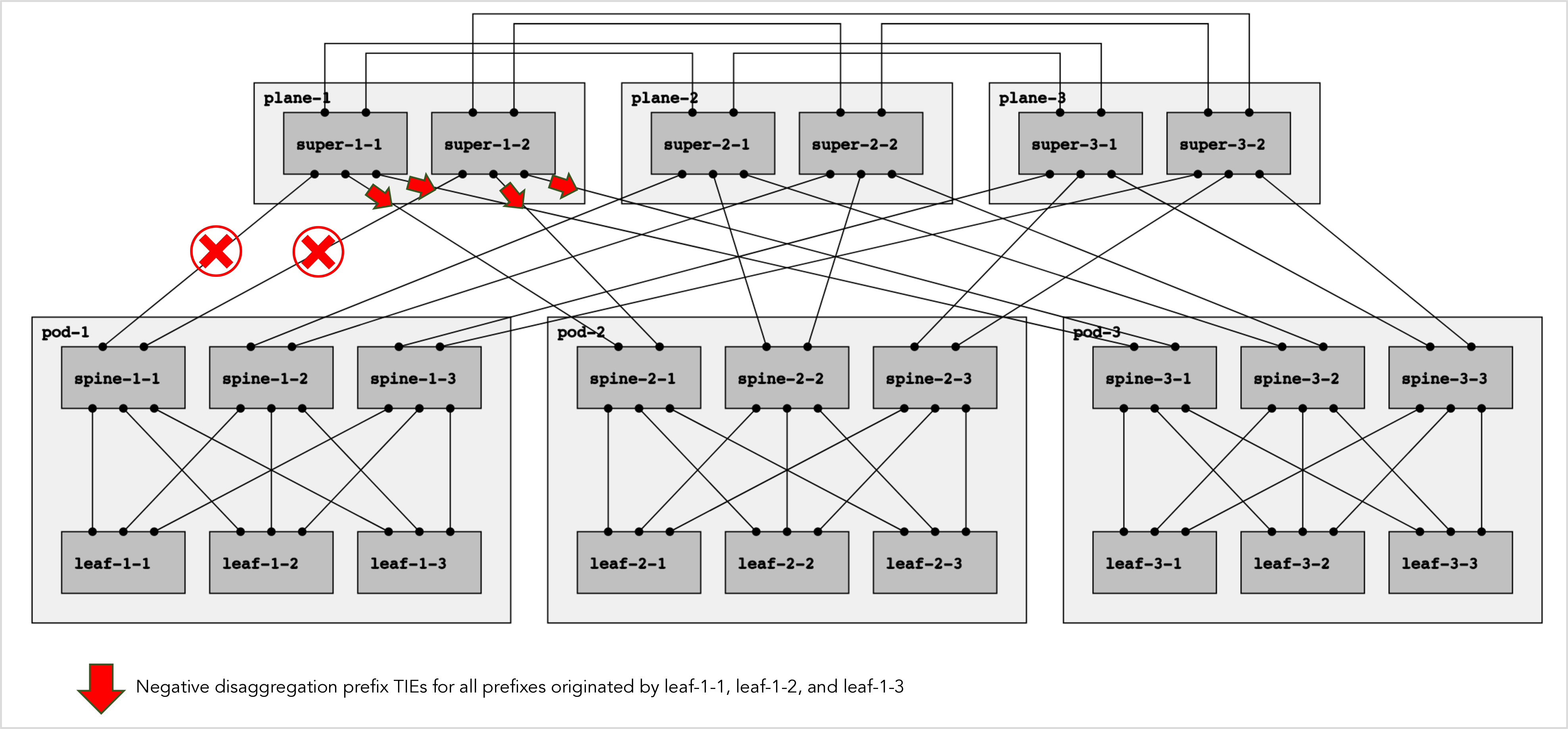
Figure 10: Originating south negative disaggregation prefix TIEs.

As suggested by its name, a negative disaggregation prefix is the exact opposite of a positive disaggregation prefix:

• When a node N advertises a positive disaggregation prefix P it is saying: “please give traffic destined for P to me instead of following the default route”. Node N is on the repair path and it is attracting traffic towards itself and away from the broken path.

• When a node N advertises a negative disaggregation prefix P it is saying: “please do not give traffic destined for P to me, if you have some other route to P prefer that other route, even if it is a less specific route such as the default route”. Node N is on the broken path and it is repelling traffic away from itself and towards the repair path.

Further below we will describe how a RIFT node installs a negative disaggregation prefix into the route table. But first we describe how negative disaggregation prefix TIEs are propagated.

Propagation of negative disaggregation

When we discussed positive disaggregation, we mentioned that positive disaggregation prefix TIEs are never propagated.

Negative disaggregation prefix TIEs, on the other hand, are propagated in certain circumstances. If, and only if, a node N receives a negative disaggregation prefix P from all of its north-bound parent nodes, then node N propagates the negative prefix P to all of its south-bound child nodes. This is shown in figure 11 below:

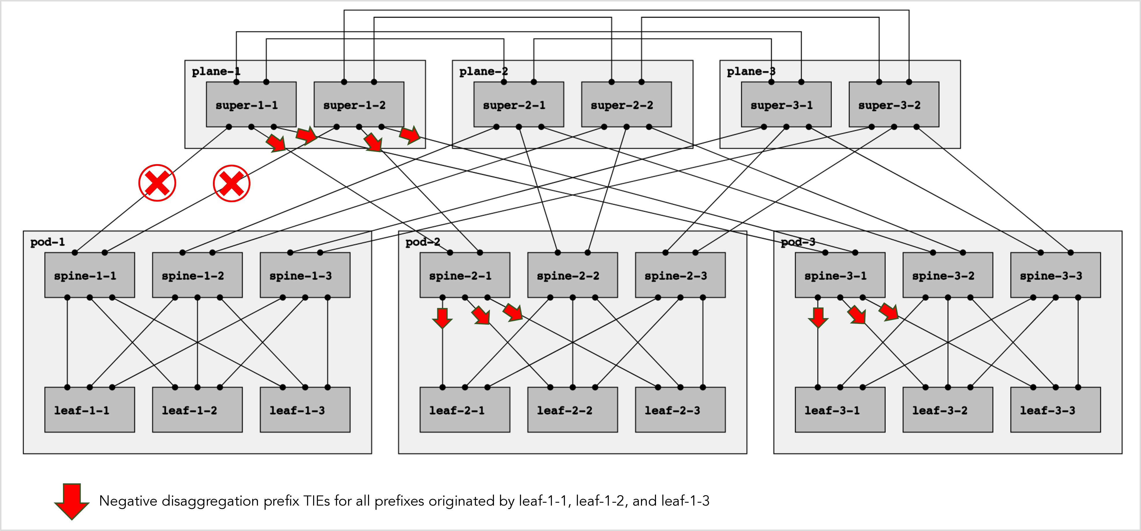
Figure 11: Propagating south negative disaggregation prefix TIEs.

Here we can see that:

• Spine-2-1 has received negative disaggregation prefixes for all the prefixes originated by leaf-1-1, leaf-1-2, and leaf-1-3.

• Spine-2-1 has received all of the negative disaggregation prefixes from both super-1-1 and super-1-2, i.e. from all of its north-bound parent nodes.

• Hence, spine-2-1 propagates all of these negative disaggregation prefixes to all of its south-bound child nodes, namely leaf-2-1, leaf-2-2, and leaf-2-3.

• For the same reason, spine-3-1 propagates all of the negative disaggregation prefixes to all of its south-bound child nodes, namely leaf-3-1, leaf-3-2, and leaf-3-3.

Storing negative disaggregation prefixes in the RIB

So far, we have explained what triggers a top-of-fabric node to originate a negative disaggregation prefix and under what circumstances a negative disaggregation prefix is propagated.

What should a node do when it receives a negative disaggregation prefix? How should a node store these negative disaggregation prefixes in the route table?

Recall what we said earlier: a negative disaggregation prefix P is used to repel traffic away from a next-hop instead of the normal behavior of “attracting” it to a next-hop. It means “don’t send traffic to this next-hop” instead of the normal behavior of “do send traffic to this next-hop”. How do we achieve this behavior in the route table?

To achieve this behavior, RIFT introduces the concept of a negative next-hop in the route table, which is more formally known as the routing information base (RIB). A negative next-hop in the RIB means don’t send the traffic to this next-hop.

Figure 12 below shows some negative next-hops (as well as some normal positive next-hops) in the RIB on leaf-2-2:

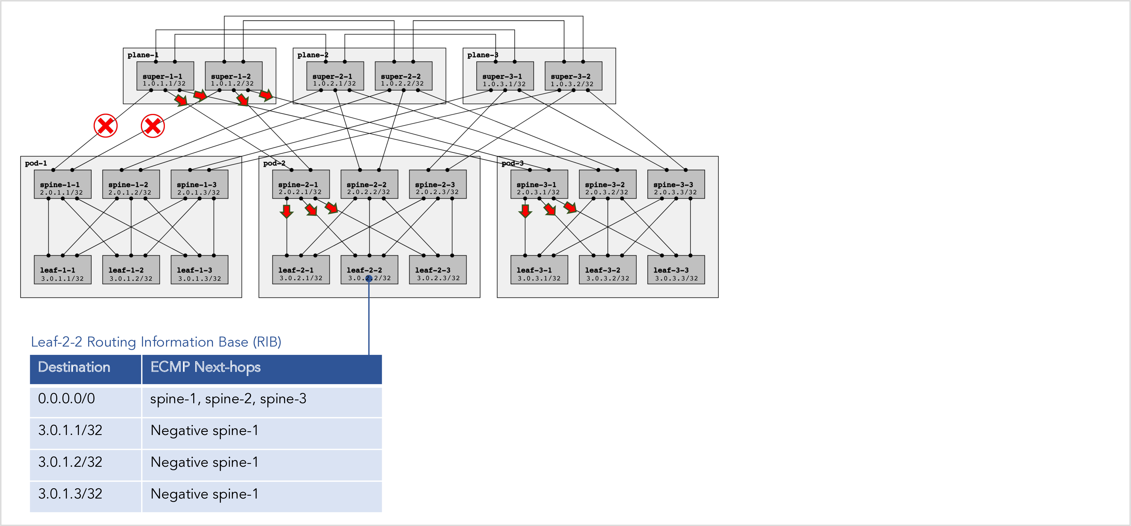
Figure 12: Routes with negative next-hops in the RIB.

An implementation may choose to only introduce the concept of negative next-hop in the RIFT local RIB as opposed to the multi-protocol global RIB that is also populated by BGP, OSPF, ISIS, RIP, static routes, etc.

Translating negative next-hops in the RIB into positive next-hops in the FIB

We have introduced the new concept of a negative next-hop in the RIB. But how is the router supposed to process a negative next-hop in the data-plane? Where is the router supposed to send the traffic to when it finds a route in the route table with a negative next-hop?

There is no such thing as a negative next-hop in router hardware, at least not in current generation hardware. So, it is necessary to translate negative next-hops in the RIB to normal (positive) next-hops when the routes are installed in the hardware forwarding table, which is also known as the forwarding information base (FIB).

The following diagram illustrates how this translation works:

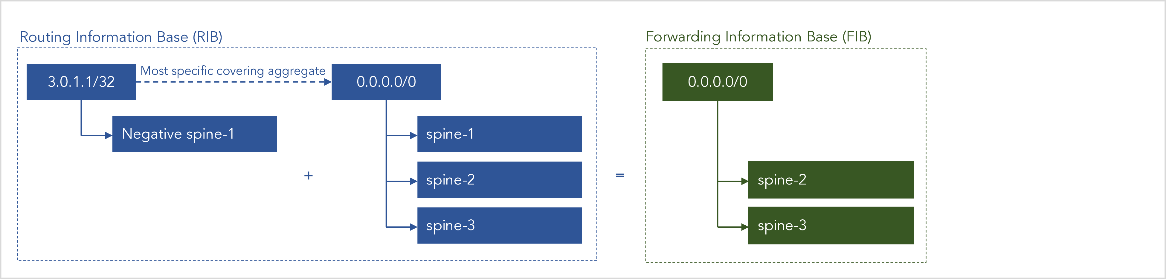
Figure 13: Translating negative next-hops in the RIB into positive next-hops in the FIB.

What is happening in this simple example is the following:

• We have a route to 3.0.1.1/32, which has a negative next-hop

• We find the most specific aggregate route that covers this route, which is the default route 0.0.0.0/0 in this case.

• We add up the next-hops of route 3.0.1.1/32 and 0.0.0.0/0, keeping in mind that a negative and positive next-hop cancel each other out.

We started with a route for 3.0.1.1/32 with negative next-hop spine-1. We translated the negative next-hop spine-1 into the complementary positive ECMP next-hops spine-2 and spine-3. These translated next-hops are stored in the FIB as shown below:

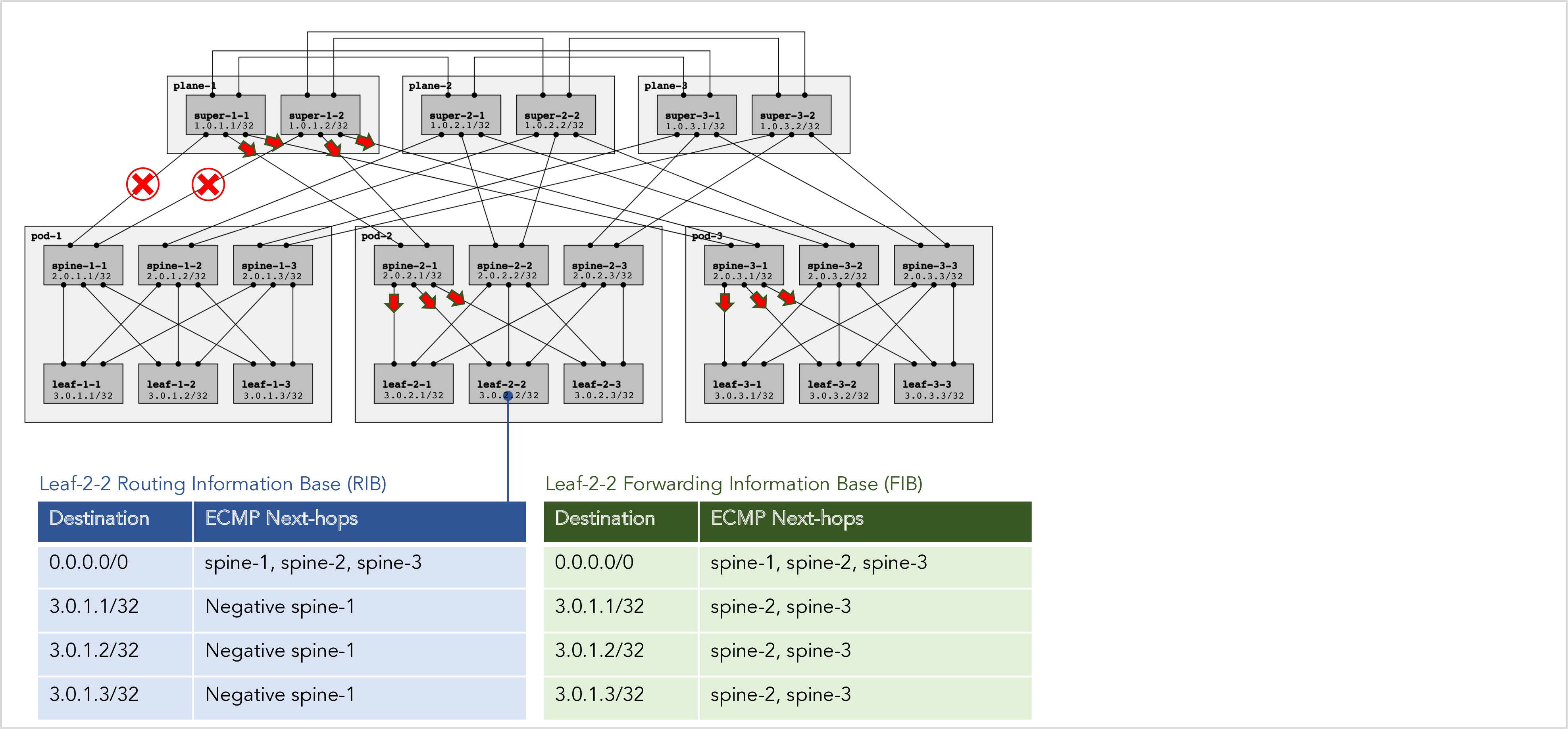
Figure 14: A RIFT RIB and FIB with negative to positive next-hop translation.

The above example is the simplest and most common scenario. Pascal Thubert gave an excellent presentation on negative disaggregation at the IETF-103 in Bangkok that describes more complex scenarios as well.