The distributed quantum Fourier transformation (DQFT) implementation in Qiskit

In this section we describe our implementation of the distributed quantum Fourier transformation in Qiskit.

What is Qiskit?

Qiskit is an open-source software development kit (SDK) for working with quantum computers at the level of pulses, circuits, and application modules. We use the following two elements of Qiskit:

• Qiskit Terra, the core component of Qiskit, which contains the building blocks for creating and working with quantum circuits, programs, and algorithms.

• Qiskit Aer which provides high-performance quantum computing simulators with realistic noise models.

Implementing the quantum Fourier transformation using Qiskit

We implement three different versions of the quantum Fourier transformation (QFT) using Qiskit:

1. A monolithic (non-distributed) version of the quantum Fourier transformation. We use this as a reference to check whether the results of the two distributed versions are correct.

2. A distributed version of the quantum Fourier transformation using teleportation.

3. A distributed version of the quantum Fourier transformation using cat states.

Installation instructions

Follow these installation instructions to install our implementation of the quantum Fourier distribution in Qiskit and the dependencies.

Directory structure

The qiskit subdirectory of this repository contains the implementation of the distributed quantum Fourier transformation in Qiskit.

There are Python modules that implement abstractions of quantum computers. The class MonolithicQuantumComputer abstracts a monolithic (non-distributed) quantum computer. The class ClusteredQuantumComputer abstracts a clustered (distributed) quantum computer.

These classes are designed in such a way that you can implement a quantum algorithm once, and then choose to run it on the monolithic or on the clustered quantum computer without any changes to the a algorithm code.

We have implemented the quantum Fourier transformation algorithm to run on these quantum computers. However, you can also implement other quantum algorithms to run on these same quantum computer classes.

File	Function
quantum_computer.py	Implements classes MonolithicQuantumComputer and ClusteredQuantumComputer
utils.py	Common utilities
examples.py	Implements examples that are used in the demonstration Jupyter notebooks

There are Python modules that implement the three flavors of quantum Fourier transformation: (1) non-distributed, (2) distributed using teleportation, and (3) distributed using cat states.

The function create_qft_circuit creates a quantum circuit that implements the quantum Fourier transformation on either a monolothic quantum computer or on a clustered quantum computer. The function takes an argument computer which can be either a MonolithicQuantumComputer or a ClusteredQuantumComputer.

The class QFT represents a monolithic quantum computer that runs the non-distributed version of the quantum Fourier transformation.

The class DistributedQFT represents a clustered quantum computer that runs the distributed version of the quantum Fourier transformation. The constructor takes a method argument which chooses between using teleportation or cat states for implementing distributed two-qubit controlled-unitary gates.

File	Function
qft.py	Implements classes QFT and DistributedQFT, and the function create_qft_circuit
test_qft.py	Unit tests for qft.py

There are also Jupyter notebooks to demonstrate the code.

File	Function
monolithic_quantum_computer.ipynb	Demonstrates class MonolithicQuantumComputer
clustered_quantum_computer.ipynb	Demonstrates class DistributedQuantumComputer
qft.ipynb	Demonstrates class QFT
teleport_distributed_qft.ipynb	Demonstrates class DistributedQFT using teleportation
cat_state_distributed_qft.ipynb	Demonstrates class DistributedQFT using cat states
density_matrices.ipynb	Some basic examples of density matrices
just_crotz.ipynb	Some basic examples of controlled rotation-Z
find_period.ipynb	An example quantum circuit for finding the period of a function

Classes that model quantum computers

Python module quantum_computer.py defines three classes that model quantum computers:

• Class QuantumComputer is an abstract base class that defines the common interface and behavior for the following two types of quantum computers.

• Class MonolithicQuantumComputer models a monolithic (i.e. non-distributed) quantum computer.

• Class ClusteredQuantumComputer models a distributed quantum computer. It is implemented as a cluster of processors connected by a entanglement-based quantum network. Each processor in the cluster is modeled by the ProcessorInClusteredQuantumComputer class.

Abstract base class QuantumComputer

The base class QuantumComputer defines the abstract operations that are used to implement a quantum algorithm. The table below lists the set of operations that is currently supported (these are all we need for implementing quantum Fourier transformations, but more operations can easily be added for other algorithms):

Function	Description
hadamard	Perform a Hadamard gate on one qubit in the circuit
controlled_phase	Perform a controlled-phase gate on two qubits in the circuit
swap	Perform a swap gate on two qubits in the circuit
set_input_number	Set the input of the circuit to a numeric value
run	Run the circuit
circuit_diagram	Display the circuit diagram
statevector_data	Return the circuit output statevector
statevector_latex	Display the circuit output statevector using LaTeX
bloch_multivector	Display the circuit output state as a Bloch multivector
density_matrix_city	Display the circuit output state as a density matrix city plot

Class MonolithicQuantumComputer

The class MonolithicQuantumComputer models a monolithic (i.e. non-distributed) quantum computer.

Under the hood, the implementation of MonolithicQuantumComputer does a simple one-to-one mapping of logical qubits to underlying concrete qubits.

Create an instance of a monolithic quantum computer:

computer = MonolithicQuantumComputer(total_nr_qubits)

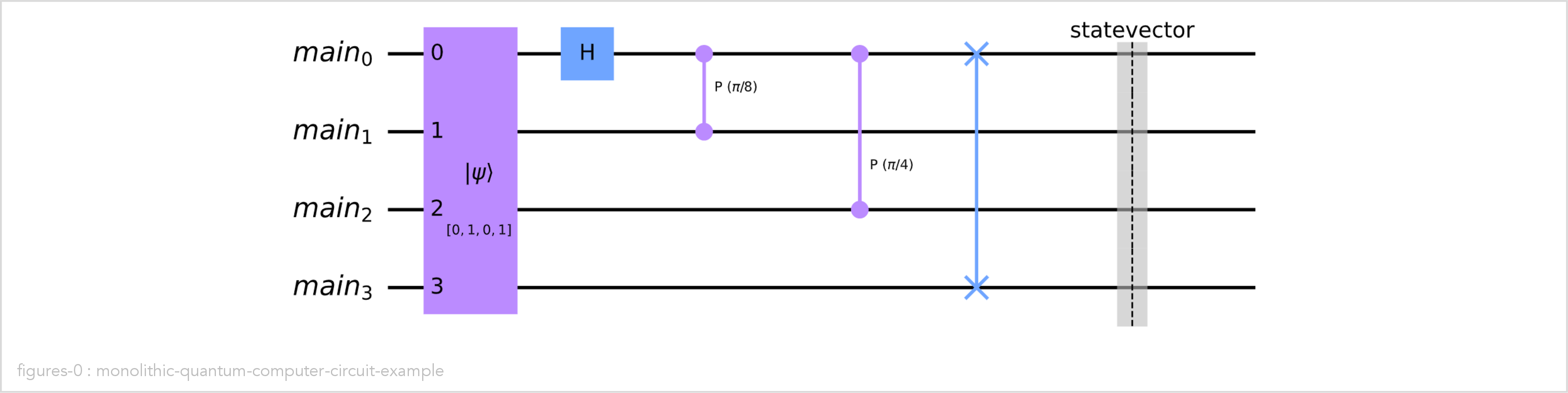
Add a few gates to the circuit:

computer.hadamard(0)
computer.controlled_phase(pi/8, 0, 1)
computer.controlled_phase(pi/4, 0, 2)
computer.swap(0, 3)

Run the circuit with input value 5 (binary 0101):

computer.run(input_number=5)

Display the circuit. Here we can see that the operations on the logical qubits are mapped one-to-one to operations on the underlying concrete qubits:

computer.circuit_diagram(with_input=True)

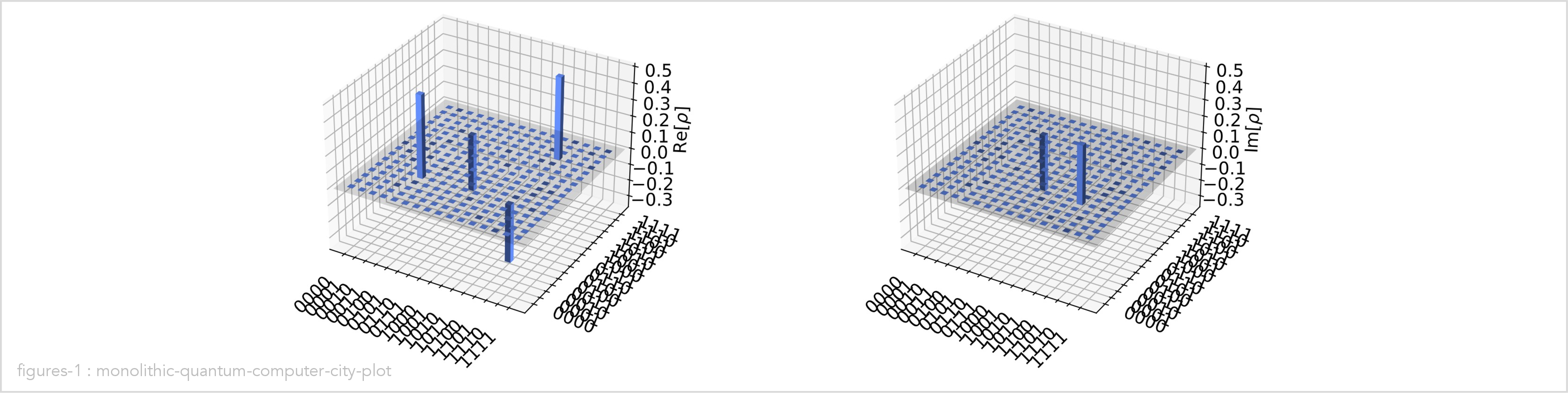
Display the output density matrix of the circuit as a city plot:

computer.density_matrix_city()

The Jupyter notebook monolithic_quantum_computer.ipynb contains a more detailed example of how to use the class MonolithicQuantumComputer.

Class ClusteredQuantumComputer

The class ClusteredQuantumComputer models a clustered (i.e. distributed) quantum computer that consists of multiple processors connected by an entanglement-based quantum interconnect.

To the quantum algorithms running on the computer, the class ClusteredQuantumComputer provides the illusion that the clustered quantum computer has a uniform set of global qubits, indexed 0 thru total_nr_qubits-1.

The algorithm can perform a single-qubit gate on any global qubit and a two-qubit gate on any pair of global qubits, without needing to worry whether those two qubits are located on the same or on different processors.

The ClusteredQuantumComputer constructor takes the following arguments:

• nr_processors: The number of quantum processors in the cluster.

• total_nr_qubits: The total number of qubits in the cluster. This must be a multiple of nr_processors so that the qubits can be evenly divided across the processors.

• method: The method that is used to implement distributed controlled-unitary gates, either Method.TELEPORT or Method.CAT_STATE

The following example creates a clustered quantum computer and defines an example circuit with some single-qubit and two-qubit gates.

nr_processors = 2
total_nr_qubits = 4
method = Method.TELEPORT
computer = ClusteredQuantumComputer(nr_processors, total_nr_qubits, method)

computer.hadamard(0)
computer.controlled_phase(pi/8, 0, 1)
computer.controlled_phase(pi/4, 0, 2)
computer.swap(0, 3)

Note that we used the exact same function calls to create the circuit as in the example for the monolithic quantum computer above. In other words, you can write a quantum algorithm once and run it either on a monolithic or distributed quantum computer without making any change to the code.

Under the hood, each processor in the cluster is modeled by a _ProcessorInClusteredQuantumComputer object. Note that the class name starts with an underscore; it is a private class used internally in the implementation that is not intended to be used by algorithm developers.

The processors are indexed 0 thru nr_processors-1.

Each processor has a set of local qubits, indexed 0 thru nr_qubits_per_processor-1 where nr_qubits_per_processor = total_nr_qubits / nr_processors.

It is very easy to map a global qubit index to a combination of a processor index and a local qubit index:

processor_index = global_qubit_index // nr_qubits_per_processor
local_qubit_index = global_qubit_index % nr_qubits_per_processor

When the ClusteredQuantumComputer is asked to perform a single qubit gate on a global qubit, it simply maps the global qubit index to a processor index and a local qubit index on that processor, and then executes the single qubit gate on that local qubit.

In the following example, we can see that global qubit index 2 is mapped to processor index 1 and local qubit index 0 (we have deleted some details from the circuit diagram that will be explained later):

computer = ClusteredQuantumComputer(nr_processors=2, total_nr_qubits=4, method=Method.TELEPORT)
computer.hadamard(2)
computer.circuit_diagram()

Things get more interesting when the ClusteredQuantumComputer is asked to perform a two-qubit gate.

First, clustered quantum computer maps the global qubit index of each involved qubit to a processor index and a local qubit index.

If both qubits happen to be mapped to the same processor, the clustered quantum computer simply executes the two qubit gate locally on that processor.

In the following example, we perform a controlled-phase operation between global qubits 2 and 3. These happen to be located on the same processor, so we can perform the gate locally on that processor.

computer = ClusteredQuantumComputer(nr_processors=2, total_nr_qubits=4, method=Method.TELEPORT)
computer.controlled_phase(pi/4, 2, 3)
computer.circuit_diagram()

If the two qubits are not located on the same processor, the clustered quantum computer implements the two qubit gate in a distributed manner.

For controlled-unitary gates (of which controlled-phase is an example), there are two different methods for implementing the gate in a distributed manner:

• Using teleportation:

  • Teleport one qubit, so that both qubits are located on the same processor.
  • Perform the two qubit gate locally on that processor.
  • Teleport the qubit back to its original processor.

• Using cat states:

  • Perform a cat-entangle operation to create an additional entangled control qubit on the same processor as the target qubit.
  • Perform the two qubit gate locally on that processor.
  • Perform a cat-disentangle operation to disentangle the additional control qubit.

For two qubit gates which are not controlled-unitary gates (e.g. a swap gate) we always use the teleportation method.

The implementation of teleportation and cat states requires some extra ancillary qubits and some classical bits to implement the communication between the processors across the quantum interconnect.

Up until now, we have omitted these ancillary quantum qubits and classical bits from the circuit diagrams. In the following example, we show the complete circuit diagram.

computer = ClusteredQuantumComputer(nr_processors=2, total_nr_qubits=4, method=Method.TELEPORT)
computer.circuit_diagram()

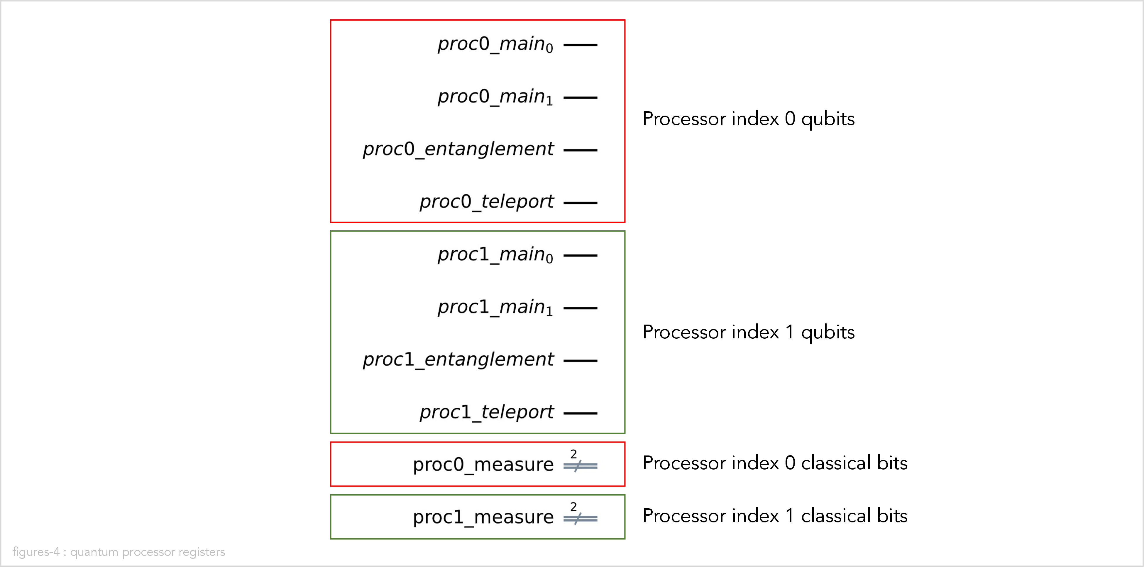
In the above circuit we have the following qubits and classical bits:

• The main qubits store the state for the quantum algorithm. There are four main qubits in total, with global indexes 0 thru 3. Each processor has two main qubits, with local indexes 0 thru 1.

• The ancillary qubits are used for quantum communication between the processors:

  • The entanglement qubit holds one half of an entanglement with another processor. The entanglement is used to teleport another qubit or to entangle a cat state.

  • The teleport qubit is used to temporarily store the sent or received qubit during teleportation.

• The classical measurement bits are used to measured classical bits during teleportation, cat state entanglement, or cat state dis-entanglement.

In the following example, we use the teleportation method to implement a controlled-phase gate between qubits 0 and 3, which are located on different processors.

computer = ClusteredQuantumComputer(nr_processors=2, total_nr_qubits=4, method=Method.TELEPORT)
computer.controlled_phase(pi/4, 0, 3)
computer.circuit_diagram()

Although, we only asked for a single controlled-phase gate, the circuit that the clustered quantum computer generates is quite complex:

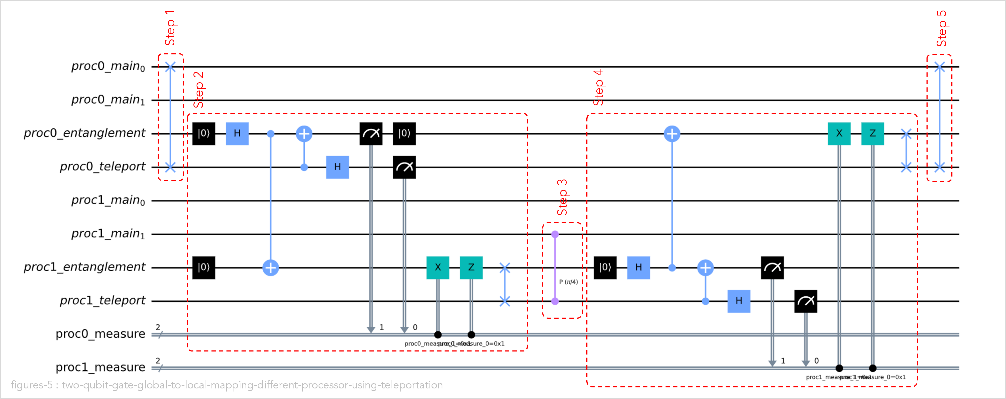
We can understand what is happening by breaking the circuit down into five steps:

• Step 1: Swap the control qubit for the controlled-phase gate (proc0_main0) into the teleport on processor 0 (proc0_teleport) in preparation for teleporting it to processor 1.

• Step 2: Teleport a qubit from processor 0 to processor 1 (proc0_teleport to proc1_teleport). Teleportation is implemented using the following sub-steps:

  • Create an entanglement (a |ɸ+> Bell state to be precise) between qubits proc0_entanglement and proc1_entanglement using a Hadamard and a controlled-NOT gate.

  • Perform two measurements on processor 0, and store the results in the proc0_measure classical register.

  • Use the classical measurement results, to perform X and Z corrections on processor 1. Note: in the Qiskit simulation, we don’t model sending of classical messages between processors. In the QNE-ADK simulation, we do.

  • Swap proc0_entanglement into proc0_teleport.

• Step 3: Perform the controlled-phase gate locally on processor 1, using the teleport qubit proc1_teleport as the control gate, and proc1_main1 as the target gate.

• Step 4: Teleport the control gate proc1_teleport on processor 1 back to proc0_teleport on processor 0. The steps are similar to step 2 above.

• Step 5: Teleport the control gate from proc0_teleport back into proc0_main0.

Note that the steps are not optimal because the implementation uses teleportation as a subroutine. For example, the very last two swaps could be combined into a single swap. We don’t attempt these optimizations in cluster computer circuit generator, because the underlying circuit compilers in Qiskit are quite good at these kinds of optimizations.

In the following example, we use the cat state method instead of the teleportation method to implement a controlled-phase gate between qubits 0 and 3:

computer = ClusteredQuantumComputer(nr_processors=2, total_nr_qubits=4, method=Method.CAT_STATE)
computer.controlled_phase(pi/4, 0, 3)
computer.circuit_diagram()

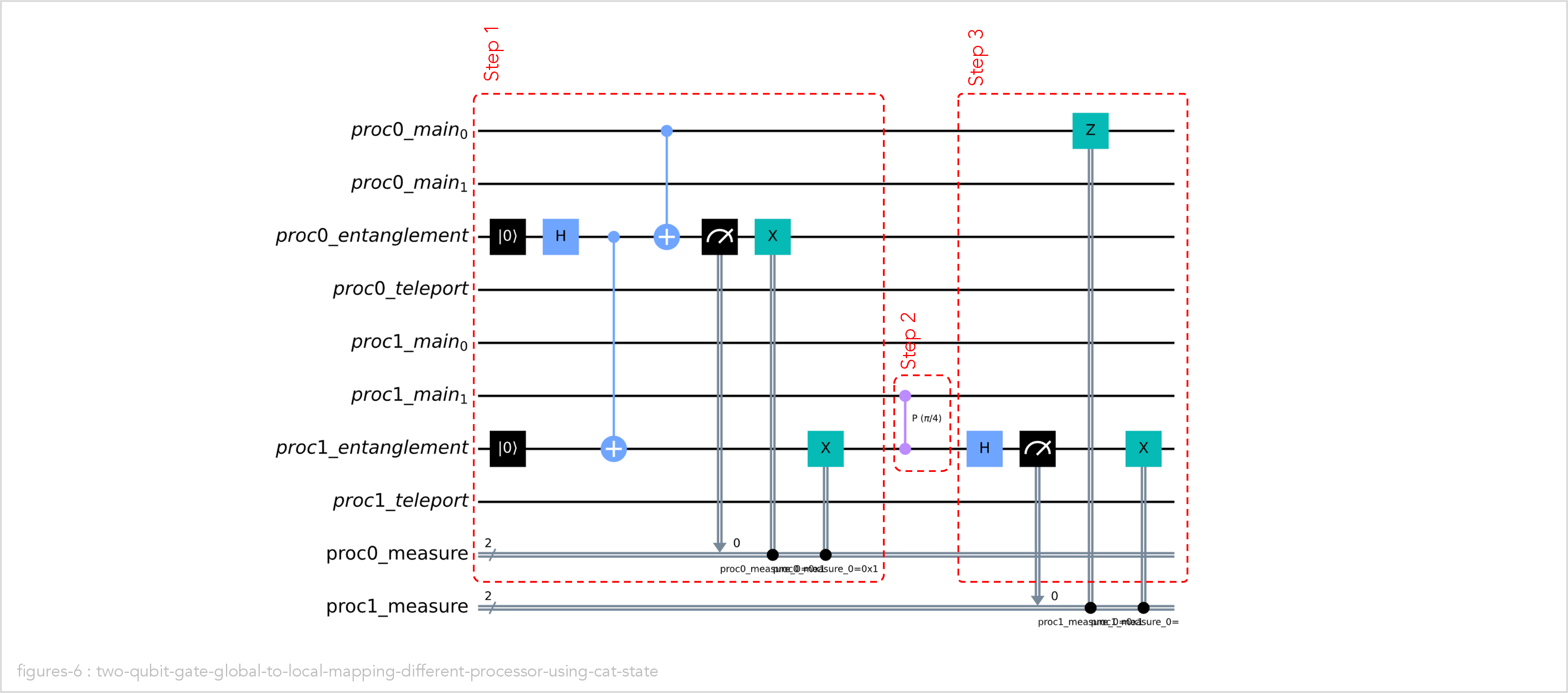
When using the cat state method to implement the distributed controlled-phase gate, we have three steps:

• Step 1: Do a cat-entanglement operation to entangle qubit proc1_entangle on processor 1 with the original control qubit proc0_main0 on processor 0.

• Step 2: Perform the controlled-phase gate locally on processor 0 between the entangled control qubit proc1_entangle and the original target qubit proc1_main1.

• Step 3: Do a cat-disentangle operation to disentangle the original control qubit proc0_main0.

As you can see, the cat state method is simpler than the teleportation method. However, we can only use if for controlled-unitary two qubit gates.

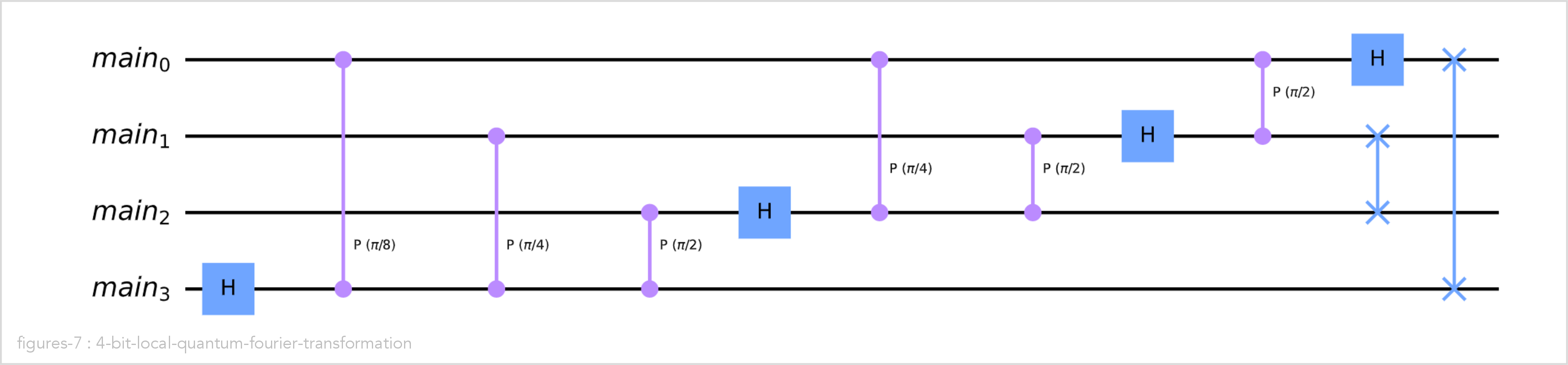
The quantum Fourier transformation algorithm

The function make_qft_circuit in Python module qft.py is responsible for generating the circuit to implement a quantum Fourier transformation.

The algorithm is essentially the same as the one presented in the quantum Fourier transformation chapter in the Qiskit textbook and it is simple enough to show the complete source code here:

def create_qft_circuit(computer, final_swaps=True):
    _create_qft_circuit_rotations(computer, computer.total_nr_qubits)
    if final_swaps:
        _create_qft_circuit_final_swaps(computer)

def _create_qft_circuit_rotations(computer, remaining_nr_qubits):
    if remaining_nr_qubits == 0:
        return
    remaining_nr_qubits -= 1
    computer.hadamard(remaining_nr_qubits)
    for qubit in range(remaining_nr_qubits):
        computer.controlled_phase(pi / 2 ** (remaining_nr_qubits - qubit), qubit, remaining_nr_qubits)
    _create_qft_circuit_rotations(computer, remaining_nr_qubits)

def _create_qft_circuit_final_swaps(computer):
    for qubit in range(computer.total_nr_qubits // 2):
        computer.swap(qubit, computer.total_nr_qubits - qubit - 1)

The create_qft_circuit does not know or care whether it is generating the circuit for a monolithic quantum computer or for a distributed quantum computer:

• If the computer argument is a MonolithicQuantumComputer object, the circuit will be generated for a monolithic quantum computer.

• If the computer argument is a ClusteredQuantumComputer object, the circuit will be generated for a clustered quantum computer. All necessary teleportations and/or cat states will automatically be generated under the hood.

The monolithic (non-distributed) quantum Fourier transformation

The class QFT is a convenience class which represents the quantum Fourier transform running on a monolithic (non-distributed) quantum computer.

The implementation is trivial:

class QFT(MonolithicQuantumComputer):

    def __init__(self, total_nr_qubits, final_swaps=True):
        MonolithicQuantumComputer.__init__(self, total_nr_qubits)
        create_qft_circuit(self, final_swaps)

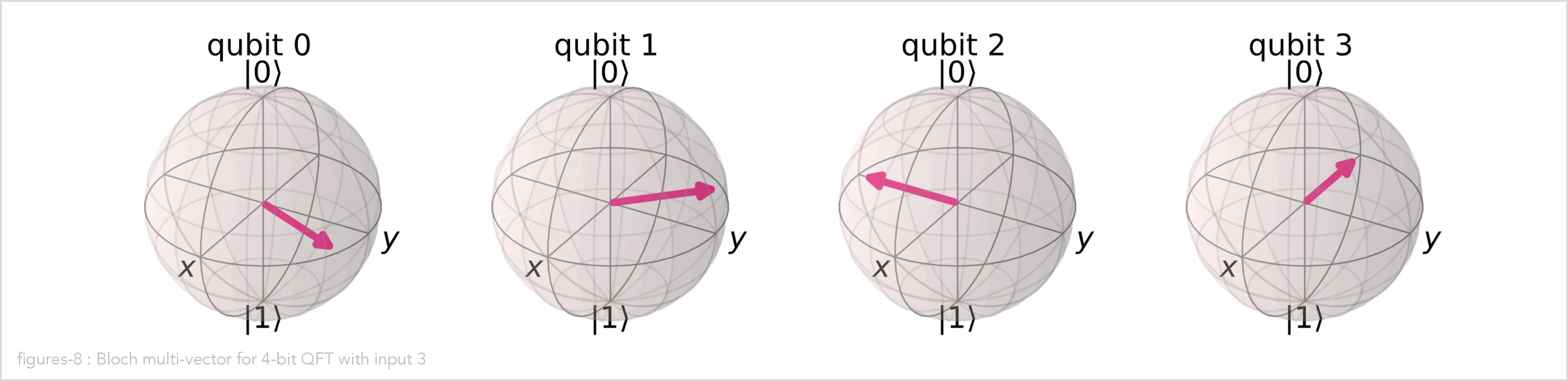
In the following example, we create a 4-qubit QFT, run it with input value 3, and show the result as Bloch spheres:

qft = QFT(total_nr_qubits=4, final_swaps=True)
qft.run(input_number=3)
qft.circuit_diagram()

qft.bloch_multivector()

The clustered (distributed) quantum Fourier transformation

The class DistributedQFT is a convenience class which represents the quantum Fourier transform running on a clustered (distributed) quantum computer.

Once again, the implementation is trivial. Note that this implementation uses the exact same create_qft_circuit function as the monolithic implementation:

class DistributedQFT(ClusteredQuantumComputer):

    def __init__(self, nr_processors, total_nr_qubits, method, final_swaps=True):
        ClusteredQuantumComputer.__init__(self, nr_processors, total_nr_qubits, method)
        create_qft_circuit(self, final_swaps)

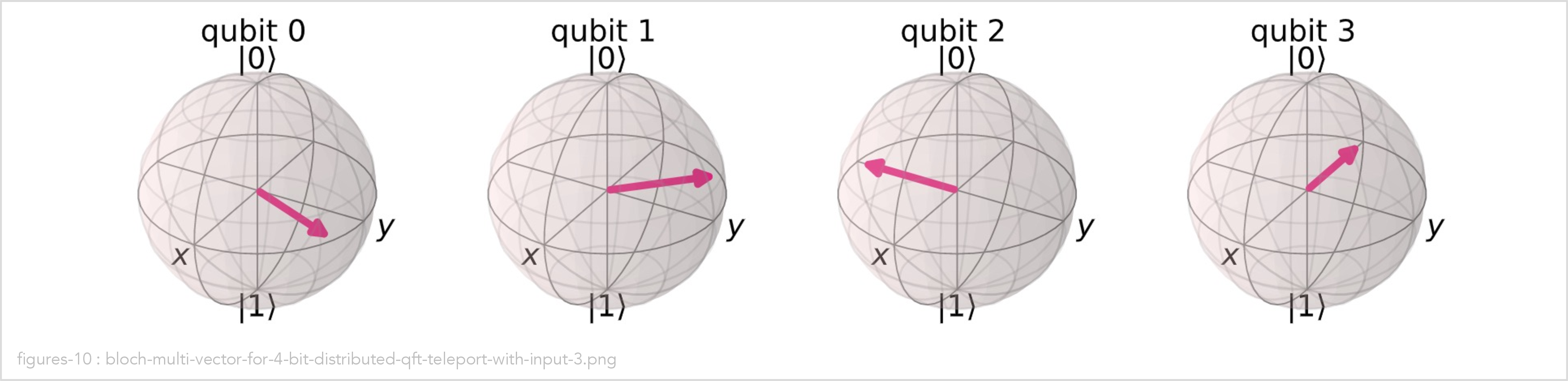
In the following example, we create a 4-qubit DistributedQFT using the teleport method, run it with input value 3, and show the result as Bloch spheres:

qft = DistributedQFT(nr_processors=2, total_nr_qubits=4, method=Method.TELEPORT)
qft.run(input_number=3)
qft.circuit_diagram()

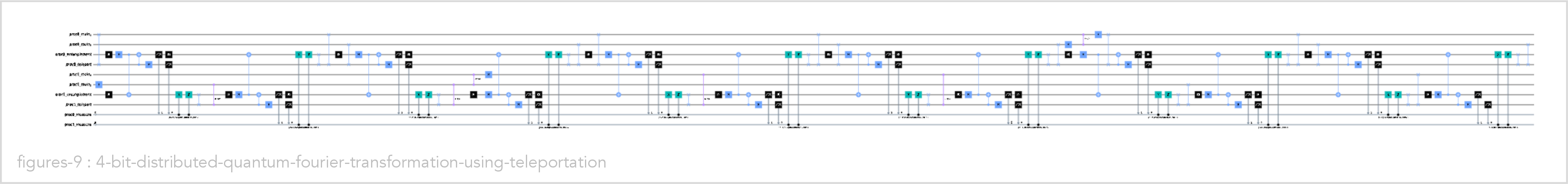
qft.bloch_multivector()

Testing the correctness of the distributed quantum Fourier implementation

If you paid close attention you may have noticed that the Bloch spheres produced by the QFT class are identical to the Bloch spheres produced by the DistributedQFT class.

This is a good thing! It means that the non-distributed and distributed implementation of the quantum Fourier transformation produce the same output states given the same input states.

If we had displayed the state vectors instead of the Bloch spheres, this would be less obvious because the state vectors produced by non-distributed and distributed implementation differ by a global phase factor which can be ignored.

The file test_qft.py contains a Pytest automated unit test which tests the correctness of our DistributedQFT class. There are several test cases, but the most important test case is test_dqft_same_as_qft. It runs the distributed quantum Fourier transformation for various numbers of qubits, various methods, and various input values. For each run, it checks whether the state vector produced by the distributed QFT is the same as the state vector produced by the non-distributed QFT for the same input value. It uses utility function state_vectors_are_same which ignores global phase differences and rounding errors when comparing state vectors.

def test_dqft_same_as_qft():
    nr_processors = 2
    test_cases = [
        (Method.TELEPORT, 2, 2, 0),
        (Method.TELEPORT, 2, 2, 1),
        (Method.TELEPORT, 2, 4, 0),
        (Method.TELEPORT, 2, 4, 3),
        (Method.TELEPORT, 2, 4, 12),
        (Method.TELEPORT, 2, 4, 15),
        (Method.TELEPORT, 2, 6, 3),
        (Method.TELEPORT, 3, 6, 11),
        (Method.CAT_STATE, 2, 4, 9),
    ]
    for method, nr_processors, total_nr_qubits, input_number in test_cases:
        qft = QFT(total_nr_qubits)
        qft.run(input_number)
        qft_statevector = qft.main_statevector()
        dqft = DistributedQFT(nr_processors, total_nr_qubits, method)
        dqft.run(input_number)
        dqft_statevector = qft.main_statevector()
        assert state_vectors_are_same(qft_statevector, dqft_statevector)

Running the unit tests indicates that our distributed QFT implementation does indeed produce the correct output states:

$ pytest -v .
================================= test session starts ==================================
platform darwin -- Python 3.8.14, pytest-7.2.0, pluggy-1.0.0 -- /Users/brunorijsman/git-personal/quantum-internet-hackathon-2022/venv/bin/python3.8
cachedir: .pytest_cache
rootdir: /Users/brunorijsman/git-personal/quantum-internet-hackathon-2022/qiskit
collected 4 items

test_qft.py::test_monolithic_qft_one_qubit PASSED                                [ 25%]
test_qft.py::test_monolithic_qft_two_qubits PASSED                               [ 50%]
test_qft.py::test_monolithic_qft_four_qubits PASSED                              [ 75%]
test_qft.py::test_dqft_same_as_qft PASSED                                        [100%]

================================== 4 passed in 2.18s ===================================